Sound Design in Web Audio: NeuroFunk Bass, Part 2

Welcome back to the second, and final, piece of this short series on sound design in Web Audio! If you haven’t been following along, I’ll recommend that you take a look at Part 1 to get a sense of where we are, and where we’re going with this article, as I’m just going to jump in right where we left off.

In the last article, we finished up with a look at the following block of code from the index.js module.

function stepOne(callback) {  
  var bass = new Bass(ctx);
  var recorder = new RecorderWrapper(ctx);
  var ws = new WaveShaper(ctx, {amount: 0.6});
  var notes = [
    ‘g#1’, ‘g#1’, ‘__’, ‘g#3’,
    ‘g#1’, ‘g#1’, ‘__’, ‘b2’,
    ‘g#1’, ‘g#1’, ‘g#1’, ‘g#1’,
    ‘__’, ‘g#2’, ‘__’, ‘c#2’
  ];

  bass.connect(ws);
  ws.connect(recorder);
  ws.connect(ctx.destination);

  recorder.start();
  bass.play(BPM, 1, notes, function(e) {
    recorder.stop(callback);
  });
}

We covered the Bass synthesizer and the WaveShaper module in the previous article, so let me call your attention to the final piece of this function body: the recorder. Each step of the process outlined in the index.js file ends with the audio graph terminating at both the output destination ctx.destination, and the recorder input. As the sound from a given step plays, the audio buffer is recorded straight into a Float32Array using Matt Diamond’s wonderful Recorderjs project. These arrays are copied into AudioBuffer objects and used to kick off function stepTwo(buffer, callback) and function stepThree(buffer, callback) in index.js. To explain why stepTwo and stepThree rely on recorded buffers rather than the real-time generator output, we now bring our discussion to the topic of resampling.

Resampling

After studying so many tutorials and explanations for creating a sound like the one we’re doing here, it seems that there is a pretty pervasive misunderstanding of resampling amongst “bedroom” producers, and maybe even several mainstream producers. Or, at least, it seems there’s a pervasive misuse of the term. So, I want to take a minute to explain exactly what resampling is before we get into what effect it has on the resulting sound.

True resampling typically deals with sample rate conversion, but in the digital signal processing (DSP) domain it can also pertain to bit depth reduction (sometimes called decimation). Imagine we have a WAV file holding a simple sine wave for 1 second at 441Hz – just above A4. Typically, WAV files, and most audio engines, use a sample rate of 44,100Hz (44.1kHz). That means that this WAV file in our example contains 44,100 sample frames, each containing a discrete value representing our continuous sine wave signal at a given point in time. Now suppose that, for whatever reason, we need to change the sample rate of our WAV file to 22,050Hz. All of a sudden we have to figure out how to fit those 100 sine wave cycles (44,100 / 441) in half the number of sample frames. One way to accomplish this would be to discard every other frame while iterating across the initial buffer, perhaps computing new discrete values by averaging or interpolating between original samples which represent our continuous signal (resampling). Clearly, this comes with a loss of quality, as where we previously had 44,100 numbers describing our signal, we now only have 22,050.

Another, perhaps more simple, example of resampling could be the case where our original WAV file uses 24 bits to represent the value of the signal in each discrete sample frame. This is a common WAV file format. Another common WAV file format uses only 16 bits for the same information. Supposing we want to convert our original 24-bit depth WAV file to a 16-bit depth WAV file, we could resample the original 44,100 sample frames, casting each value to the new 16-bit data type, again resulting in a loss of quality. Both this example and the previous example are specifically examples of downsampling, of which quality loss is characteristic, however there also exists upsampling, which attempts to increase the audio quality by interpolating between successive values.

Now that we have a proper definition of resampling is, let’s take a step back and look at stepTwo in index.js to identify the resampling process. You’ll find that towards the top of the stepTwo function body exists these two assignment statements:

  var s1 = new Sampler(ctx, buffer);
  var s2 = new Sampler(ctx, buffer, {detune: 3});

In stepTwo, these are the only instruments which generate sound – everything else simply modifies the sound as it moves through the audio graph. The Sampler object (lib/generators/Sampler.js) is a simple wrapper around the standard AudioBufferSourceNode for playing back a buffer. This abstraction is little more than the following three lines of code:

this.source = ctx.createBufferSource();
this.buffer = buffer;
this.source.buffer = buffer;

If you look a little more closely at this file, you’ll quickly notice that neither the use of s1 nor the use of s2 in stepTwo explicitly resample the provided buffer. It takes a bit of digging, but it turns out that, at least in Chromium, the implementation of detune on the AudioBufferSourceNode uses real-time resampling (see the implementation of AudioBufferSourceHandler::renderFromBuffer in AudioBufferSourceNode.cpp). This is actually a common method of implementing detune on fixed buffers; the value of the detune parameter is used to compute the playback rate of the audio buffer, which determines how quickly the implementation iterates over the buffer when writing data to the output buffer. In our case of increasing the pitch +3 cents, the implementation steps through the buffer in increments of 1.0017. Thus when the floating sum wraps around, skipping an integer value, we skip a frame and interpolate with its value to write the next output buffer sample frame. So where the original buffer uses N frames to hold our recording, playing it back at +3 cents uses M frames, where M = N / playbackRate = N / 1.0017. Therefore, setting a detune of +3 cents on s1 results in real-time downsampling as the buffer is written to its output.

At this point, we understand what resampling is, and how Chromium’s Web Audio implementation is doing it in the context of our example, but we haven’t talked about what it’s actually doing to the sound we’re making. Playing the recorded sample from stepOne and a duplicate of the sample sample at +3 cents is a hassle; couldn’t we just introduce another two saw wave oscillators with the appropriate detune values and run it through the same audio graph? If there’s any one question which pulled me down the rabbit hole that led to this project, this is it. Fortunately, we’re already really close to the answer, but to get the rest of the way there we have to look at phasing again in the context of this new resampling knowledge.

Let's step back again to look at this resampling process on a single sine wave:

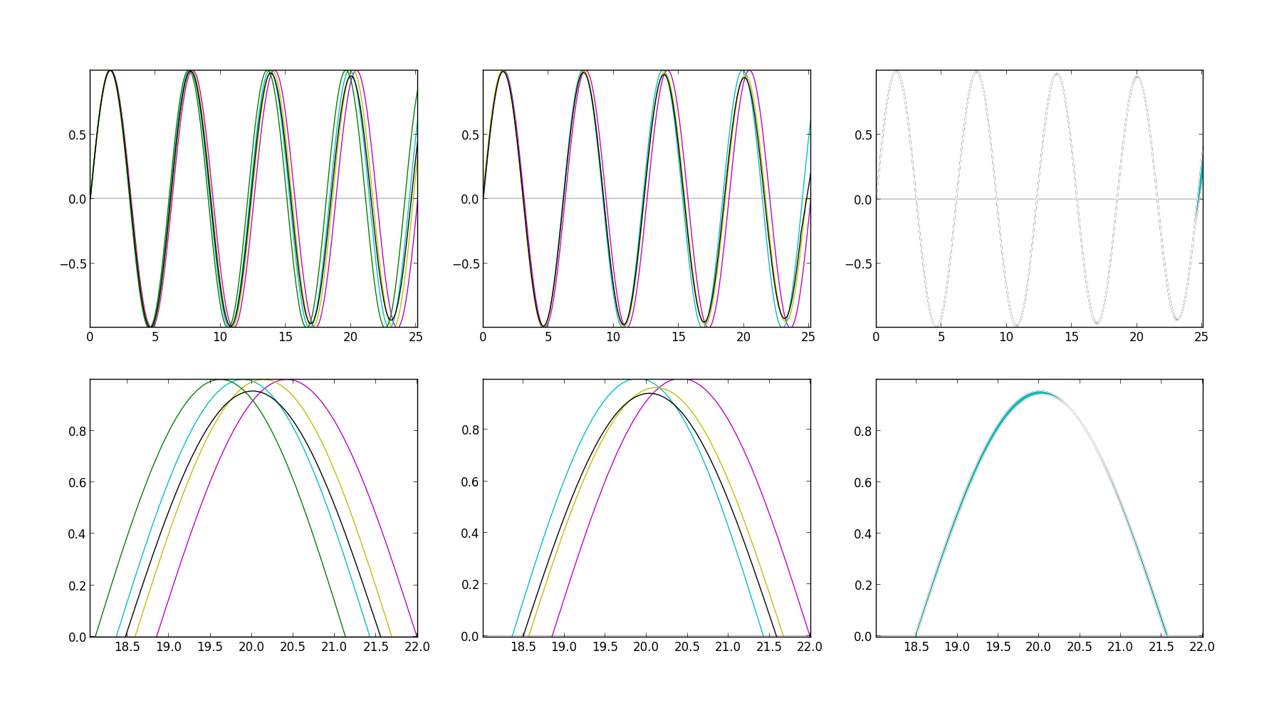
The top left graph in this figure represents four cycles of a pure sine wave played at 440Hz (magenta), next to the same sine wave played at 440 * 1.0265 (cyan), which accounts for our detuneRatio in the Bass module. These waves are then duplicated and drawn again with a detune of +24 cents (my audio implementation uses a +3 cents detune, but here the exaggerated value helps draw useful graphs). Finally, their scaled sum is drawn in black. Below, in the bottom left, you'll find a zoomed in region of the same graph. Note that the X axis here represents time on a scale different from 1:1. This leftmost plot draws what we would expect in the case of trying to implement stepTwo without resampling – that is, just by adding additional oscillators with the right detune value.

The graph to its right (top middle) shows the same waves, except that the wave drawn in yellow represents the sum of the magenta and cyan lines (our original generator sound) resampled by the same process Chromium uses to reflect a +24 cents detune. The black line again shows the scaled sum of the other three waves, and the graph beneath it (bottom middle) shows the zoomed in region. Studying these four graphs, you might struggle to identify the difference between the resampling approach and the raw approach. Indeed, the difference we're interested in is extremely slight in the visual representation.

The graph in the top right draws the difference between the black line in the first graph and the black line in the second graph (the lines which represent our final signal, with and without the resampling step). Beneath that (bottom right) you'll find another zoomed in region of the same graph. The blue region drawn here represents the different phasing characteristics of our signals. During the resampling step, as we step through the initial sine wave buffer, downsampling to reflect the detune amount, we lose important information about the continuous signal we're trying to emulate. We make guesses about that information by interpolating between successive sample frames so that when we drop a frame we don't have a discontinuity in our signal. It's extremely slight, but those guesses are wrong enough to introduce phase artifacts in the resampled signal, which, when played back next to the original sample changes the phasing characteristics of the two signals interacting. This is what we're seeing in blue on the rightmost graphs. We are examining this effect in the context of one sine wave here, but now remember that our saw wave harmonics are sine waves. So these tiny changes happen with tiny variations all across the frequency spectrum – on each harmonic of our bass sound – and thus produce a very audible effect. Depending on the detune amount, this effect is a tighter, zip-like phasing characteristic that I have not been able to reproduce just by duplicating the oscillators.

Interestingly, I attribute a lot of the earlier neurofunk bass sounds to this tiny detail of resampling. Actually, groups like Noisia and Evol Intent have shared that this exact resampling process is one which they repeat over and over again until they have a result they find interesting.

Putting It All Together

We've now covered phasing, wave shaping, and resampling in great detail. These are perhaps the most important pieces of this process, and certainly the pieces which I understood the least before embarking on this project. The remainder of the process is nothing more than a creative, repetitive application of these concepts. Create a sound, shape it, resample it, repeat. For that reason, I will be deliberately brief with the remainder of this article. We'll quickly walk through the last few bits of the code to finish the example, and then wrap up with a bit of anecdotal advice for using these kinds of sounds in your compositions.

The remainder of stepTwo simply brings our bass to life by shaping the sound and introducing more movement.

// Merge the duplicate buffers
s1.connect(m1);
s2.connect(m1);

// Connect the left side of the parallel chain
m1.connect(bp.input);
bp.connect(notch);
notch.connect(cr);
cr.connect(m2);

// Connect the right side of the parallel chain
m1.connect(m2);

This is one of my favorite ways of adding movement in this step. We merge s1 and s2 through a gain node (m1), then split off the signal, sending one end through a bandpass filter, then a notch filter, then a chorus module, and finally mix it into m2 with the dry signal from m1. Sometimes I find it really interesting to pan one side of the chain left, and the other side right, before mixing them back together, which can really open up the stereo width of the sound, making the high end characteristics of our bass that much more interesting. The fun part, however, comes from automating the frequency parameter of the bandpass and notch filters.

function scheduleFilterAutomation(param, steps, rand) {
  var beats = 4;
  var duration = (60 / BPM) * beats;
  var interval = duration / steps;

  param.setValueAtTime(rand(), ctx.currentTime);

  for (var i = 0; i < steps; i++) {
    var delta = (i + 1) * interval;
    var t = ctx.currentTime + delta;

    param.exponentialRampToValueAtTime(rand(), t);
  }
}

  scheduleFilterAutomation(
    bp._filter.frequency,
    8,
    makeRandomGenerator(80, 18000, 3)
  );

Because this is code, and introducing randomness into the sound design process yields interesting results, I couldn't help but want to randomly modulate these filters. As a result, each time you run the demonstration, the movement introduced in stepTwo ought to change. In the code block shown above, makeRandomGenerator is a simple function which returns a separate function, which produces random values between the supplied range, weighted towards the lower end of the range by the third argument.

This step ends by running m2 through another chain of effects. I've used a set of filters just to touch up (equalize) the sound, another WaveShaper to give even more of an edge, a compressor to help tighten everything up, and finally another bandpass filter in parallel with a lowpass filter. Similar to the previous bandpass and notch filters, I randomly modulate the frequency parameter on these filters as well. This is the piece of the process which I so deliberately identified in KOAN Sound's "Starlite" in the previous post – the lowpass filter movement seemingly attempting to "restrain" the bass we've made so far. In a proper composition, it would be unlikely to use randomness in the automation of this filter's parameters, but here it was an interesting experiment.

Finally, stepThree takes all of our progress thus far, and applies the resampling process again in the same way, followed by one final WaveShaper, and one final lowpass filter just to soften the very high end of our sound. The final result is what you'll hear in the third iteration of the sound when you run the demonstration.

In closing, as we've now finished our exploration through this sound design process, I want to remind you that so many pieces of this process are variables waiting to be tweaked. Many of the producers pushing this style of music have shared that this process is simply a labor of love. It takes a lot of time, and often, much of the result is thrown out as only certain slices of the sound make their way into a final track. Finding a piece of your sound here to rhythmically layer with a different bass instrument can provide really great results.

Go on and make great bass!