Introduction to Oversampling for Alias Reduction
Oversampling is the process of sampling a signal with a sample rate significantly higher than the Nyquist rate, where the Nyquist rate is defined as twice the highest frequency component in the signal. In a musical context, it's often used for avoiding aliasing, but has additional properties that make it applicable to several use cases.
As I started getting my head into the world of digital signal processing, one of my first projects was waveshaping distortion. It seemed simple enough at first: construct a function f(x) such that your output signal is the result of applying f to your input signal: output(t) = f(input(t)). A popular choice for subtle clipping, for example, is f(x) = tanh(x).
I didn't get very far before bumping into this topic of oversampling. This was the first topic that I encountered that just really threw me for a loop. Before you can begin to understand oversampling, you must first understand certain fundamentals of digital signal processing. Then you must understand when and how oversampling can play a role, and how to implement it, all of which can be really complicated for a beginner in the field.
So, here I want to introduce you to oversampling in the context of music DSP, in the way that I've come to understand it. We'll cover each of the fundamental concepts that play a role in a comprehensive understanding of the oversampling process, work through a naive implementation, and make considerations for a more optimized, production-level algorithm.
Sample Rates, Nyquist, and Aliasing
You'll notice above that even in trying to define oversampling, I touched on another concept that we need to understand: the Nyquist rate. In digital signal processing, we do our best to represent continuous signals with discrete sample points. The Nyquist-Shannon sampling theorem, [1] which essentially governs how to accurately represent a continuous signal in discrete time, states that we can perfectly reconstruct a continuous signal, s(t), which contains frequencies no higher than N hertz, by a series of samples spaced 1/2N apart.
In the music DSP context, this often accounts for the choice of a sample rate, fs, of 44.1kHz: on average, the human hearing range is roughly 20Hz to 20kHz, thus with a sampling rate of 44.1kHz we can perfectly represent a signal, in discrete time, whose highest frequency component is less than fs/2, or 22050Hz – the top end of the human hearing range with a little room to breathe. This limit, N, or fs/2, is called the Nyquist frequency, while 2N, or fs, the Nyquist rate, determines a sufficient sampling frequency for a given signal bandwidth.
I find it helpful to think about this intuitively as well. Consider the simplest case, a sine wave at the low end of the frequency spectrum (20Hz to 20kHz). At a sample rate of 44.1kHz, we have many samples per cycle of the given sine wave. If I were to draw dots on a piece of paper to illustrate these sample points, I imagine you'd have an easy time drawing a sine wave through the sequence of dots. Consider, then, a sine wave at the high end of the frequency spectrum with the same sampling rate. Here we're close to only two samples per cycle: roughly one dot to show you the top of the sine wave and one dot to show you the bottom. It would be a little harder this time, but I think you could still draw the right curve through the provided dots. Finally, suppose we take a sine wave higher than Nyquist. At this point, we don't even have two samples per cycle. I could draw the dots on a piece of paper, but are you confident you could draw the right curve through them?
So here we hit the last important piece of the sampling theorem in our quest to understand oversampling: aliasing. In signal processing, aliasing refers to the case where two different signals become indistinguishable from one another when sampled. [2]

Let's consider that last example again: you have a series of dots in front of you on a piece of paper, equally spaced along the time axis. You could draw one sine wave at a very high frequency through those dots, knowing that I had suggested this sine wave was above Nyquist. But you could draw a different sine wave through those same sample points: a slower sine wave, and both of them are correct answers.
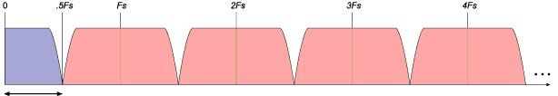
It turns out that sampling a continuous signal, even with a sufficient Nyquist rate, creates upper and lower sidebands in the discrete signal: mirrored copies of the original signal at repeating intervals related to the Nyquist rate. That is to say that in a sampled signal, we have multiple sets of "right answers" at the same time to fit the given sample points. This figure above, borrowed from the wonderful EarLevel Engineering blog, [3] shows an input signal bandwidth (the frequency range that we care about) in purple from 0Hz to fs/2, which for our purposes we could imagine is 0Hz to 22050Hz, and then shows the mirrored copies up through several integer multiples of the sampling rate, fs.
Often, this mirroring is a harmless consequence of the sampling theorem. By the time the signal reaches the DAC (Digital Audio Converter) in your audio interface, the signal we care about is still in the appropriate range. However, we run into trouble when something we do to the input signal produces new frequency content above the Nyquist frequency. While we're still in the digital domain, that higher frequency becomes indistinguishable from the same frequency mirrored about Nyquist, and by the time the signal gets to the DAC, we'd have no idea that the alias wasn't meant to be there: we've just produced a frequency component in our signal that we didn't mean to.
Nonlinear Processes
At this point, we've covered the fundamental concepts that underly the discussion of oversampling. Next we'll look at how oversampling helps avoid aliasing and how to implement it, but before we get there we should consider at least one situation where you might want to use oversampling.
As I mentioned, the way that I found myself in this rabbit hole was with waveshaping distortion. The example I gave for soft clipping, output(t) = f(input(t)) where f(x) = tanh(x), is an example of a nonlinear process: the output signal is not linearly related to the input. By contrast, a simple linear process might be f(x) = 2*x, which is roughly equivalent to adding +6dB of gain to the input signal.
A linear process such as the one above exactly preserves the wave shape of a given signal, modifying only the amplitude (and/or a translation along the Y-Axis, but we'll ignore that as it is usually undesirable and removed with a DC Blocking filter at some point in the signal chain). But a nonlinear process does not have that same property: it produces a distorted version of the input wave shape, yielding additional harmonics in the signal that contribute to the new wave shape. For example, the figure below shows the resulting frequency spectrum of taking a simple sine wave through a wave shaping function very similar to f(x) = tanh(x). Note the new harmonics.
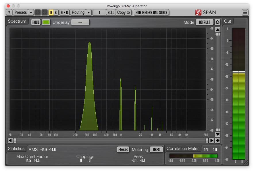
Now we have a situation where we need to consider aliasing. For example, imagine a sine wave input signal with a frequency of 18,000Hz. If we push that sine wave through a nonlinear function like the one shown above, we'll introduce new harmonics above 18,000Hz, and based on the choice of nonlinear function we may well introduce harmonics above fs/2. But because we're still in the digital domain, those new harmonics will be indistinguishable from the the same harmonics reflected about fs, potentially creating inharmonic content: a characteristic we probably don't want for a clean soft clipping algorithm.
Listening for Aliasing
We briefly covered one example where aliasing might be something to think about, but there are plenty more cases and, in some, the aliasing produces a very desirable sound. For example, the distinctly characteristic bitcrush effect relies on the aliasing introduced from low quality sample rate reduction for its characteristic sound. The classic Moog lowpass ladder filter will alias just a bit for certain input signals, and I've seen several developers leave that aliasing in their implementation as they prefer it.
Ultimately it will be up to you to identify when some of your signal processing is introducing aliasing, and whether or not you find it undesirable. One way that I like to test for aliasing is just to sweep a loud sine wave from 20Hz to 20kHz through my algorithm. If the only sounds I hear are sweeping upwards, then nothing is aliasing. Once you hear something start to sweep downwards in pitch, you can be sure that your process has started producing frequencies in the mirrored sideband of your input signal, and they're reflecting back into the audible range.
It may be helpful to plot the result with a spectrum analyser and watch the peaks as well. For some processes, you may see peaks sweeping downward that have a very small gain, say -96dB (the 16-bit noise floor), in which case maybe they're inaudible enough that you needn't worry about them. Again, in this case it will be up to you about how to proceed.
Oversampling to the Rescue
Ok, we now understand the fundamentals of digital sampling, and have an example nonlinear process which could produce aliasing. Finally, we're ready to dive into oversampling as a means of avoiding (or mitigating) the aliasing.
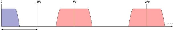
Given the context we now have, the basic procedure for oversampling is quite simple: we want to increase the sample rate of our signal, which increases the Nyquist frequency, thereby increasing the bandwidth of the signal. Then, we can run our nonlinear process and introduce harmonics with plenty more headroom before we have to worry about pushing a frequency component past our new Nyquist. Afterwards, we can run a lowpass filter on our new signal at the original Nyquist frequency, and then reduce the sample rate back to the original without leaving any frequency components in the mirrored range. Recall our visual of a sampled signal from above:
The goal of oversampling is to give that purple region (the signal bandwidth) more room before bumping into fs/2, thus giving us more headroom to run our processes before we cross into the mirrored region. For example, oversampling by a factor of 2 should double fs, and thereby double fs/2 (image credit again goes to the EarLevel Engineering blog):
Now, we can still use soft clipping on an 18000kHz sine wave, and we will potentially produce partials above 22050Hz, but because of the new sample rate those partials will not be mirrored back into the audible range. The last step then is to make sure to lowpass filter those partials out, because if they're still there when we bring the sample rate back to its original value, they'll alias in the audible range just as if we hadn't oversampled in the first place.
Naive Oversampling Implementation
We have the theory! How about the implementation? It turns out that the naive implementation is fairly straightforward as well. The first step is to insert zeros in between every sample in the input buffer:
for (int i = 0; i < numInputSamples; ++i)
{
  oversampledBuffer[i << 1] = inputBuffer[i];
  oversampledBuffer[(i << 1) + 1] = 0.;
}
Easy enough. Now our oversampled buffer has twice as many samples as our input buffer– we've doubled our sample rate! But there's a catch here. Inserting one zero between each sample in the input buffer does indeed increase the sample rate, and therefore the Nyquist frequency, by a factor of 2, but it doesn't address the mirrored component of our original signal. We've moved the goalposts, but haven't touched the signal: [4]
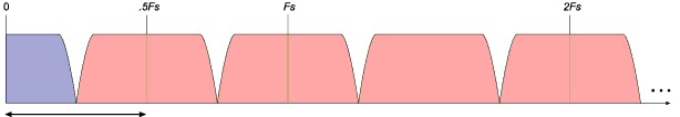
This leads to our next step: we need a lowpass filter at the original Nyquist frequency, which is now fs/4, to remove the mirrored component of the original signal from the bandwidth region that we're now working in. For the sake of this section, let's assume this is an arbitrary, simple lowpass filter, for which I will omit the implementation. (In the following section I will cover considerations for choosing a proper filter.) Now, after the filter, we have exactly the headroom we were looking for to run our nonlinear process:
As stated in the previous section, we suspect (or we have measured) that our nonlinear process will introduce frequency components above what is now fs/4. So after running said process, if we just move the goalposts back without addressing those frequency components, we'll still have aliasing. Thus we now use the same lowpass filter at fs/4 that we used after the zero padding to keep our desired signal within the original bandwidth.
Finally, we can downsample from the oversampled buffer to the original output buffer:
for (int i = 0; i < numOutputSamples; ++i)
  outputBuffer[i] = oversampledBuffer[i << 1];
This step is equivalent to a first-order hold on the oversampled signal: what would be a crude step if we hadn't taken care to use the lowpass filter beforehand.
To briefly recap, then, our naive oversampling implementation steps are:
- Insert zeros between input samples
- Lowpass filter at what is now
fs/4 - Run your nonlinear process
- Repeat the lowpass filter from step 2
- First order hold into the output buffer
What we've covered here is only 2x oversampling (oversampling by a factor of 2). For more aggressive nonlinear processes, such as sine foldback wave shaping, we need to oversample by larger factors to fully mitigate the aliasing. Luckily, we can repeat the process above multiple times for higher order oversampling. That is, for 4x oversampling, we cascade two 2x upsampling stages and two 2x downsampling stages, and so on:
- Insert zeros between input samples
- Lowpass filter at what is now
fs/4 - Insert zeros between input samples
- Lowpass filter at what is now
fs/8 - Run your nonlinear process
- Repeat the lowpass filter from step 4
- First order hold into the first oversampling buffer
- Repeat the lowpass filter from step 2
- First order hold into the output buffer
I should comment here with a reminder that this is only an introduction to oversampling. There are plenty of multi-stage approaches which use different filter designs for the different stages, and rightfully so. Meanwhile, there are many single-stage approaches for higher order oversampling with FIR filter convolution. I will leave the exploration of such topics to the reader.
Filter Design and Considerations
We made it! If you've stuck with me this far, you're a champion. There's one more important step here: choosing a proper lowpass filter. Now, I am not an expert in the various filter design choices here, but I can at least give you an introduction to the topic.
We know now that we need a lowpass filter for the upsampling and downsampling stages, but what kind of filter? In general, we want a filter with minimal passband ripple, a steep transition band (which we can usually get from higher order filters), and heavy stopband attenuation (say, at least -96dB). There are several types of filters that can offer that, and by and large, the tradeoffs to consider between them involve phase response in the passband, amount of attenuation in the stopband, and processing efficiency.
Generally there are a two main categories of filter choices here: linear phase FIR, and polyphase IIR. Usually, linear phase is an enjoyable property, as distorting the phase of a signal can, for example, smear the transients. However, implementing it can be quite costly and it can introduce a nontrivial group delay into the output signal. Polyphase IIR filters are often much more computationally efficient, decompose well into smaller order filters (i.e. a cascade of second order sections, which further aids the computational efficiency and numerical accuracy), and can be designed with properties not far from that of a linear phase FIR. For an excellent resource on what exactly is a polyphase filter, see this article from the DSP Related blog: https://www.dsprelated.com/showarticle/191.php.
It will be up to your design constraints and your product requirements to correctly choose an appropriate filter design. I'll also recommend reading the Matlab documentation for a wonderful resource on designing such filters: https://www.mathworks.com/help/dsp/examples/iir-polyphase-filter-design.html.
An Additional Use Case for Oversampling
Before I conclude this article, I want to briefly mention another application of oversampling in the music DSP context: correcting or improving a filter's frequency response.
A frequent topic in the implementation of digital filters (these can be anything, like the classic RBJ biquad filters that are still a popular choice for EQs, for example) is the use of the bilinear transform for mapping the analog frequency domain onto the digital frequency domain. It turns out that this mapping, paired with certain other details of your implementation – like the filter topology, the use of sample delays in your feedback paths, etc – can often warp the freqeuncy response of your filter especially as it approaches the Nyquist frequency. Thus, for example, at high cutoff values, your lowpass filter might start behaving differently than you would expect (maybe it starts to roll off too quickly, or not quickly enough).
There are ways to address this sort of problem by considering the underlying topology, but you can also mitigate this problem through the use of oversampling. Going back to what we learned earlier, by giving our signal more headroom (moving the Nyquist frequency away), we can roughly push that warping behavior off into the inaudible part of the spectrum. This way your filter's frequency response is more accurate on the range that you care about.
Conclusion
So now we've finished our introductory look at the use of oversampling in the music DSP context with a focus on mitigating aliasing. We've covered the fundamental concepts that play a role in the oversampling process, explored a naive implementation, and left considerations for proper filter design.
You can see why this topic might be a lot to take in for a beginner! I hope this article has given you the tools to be able to understand and evaluate when to choose an oversampling algorithm, and a strong enough grasp on the basics to be able to explore the complexities of more advanced oversampling filters.
http://www.earlevel.com/main/2007/07/03/sample-rate-conversion/ ↩︎
To understand why the insertion of zeros successfully increases the sampling rate without modifying the signal, it's useful to remember that in the digital domain we're working with the pulse-amplitude modulated form of the continuous signal. Ideal reconstruction of a continuous signal from the pulse-amplitude modulated form can be done with ideal sinc interpolation (replacing each sample point with a sinc function whose amplitude is scaled by that sample point's value, and summing the result). Thus inserting zeros does not introduce additional sinc points, therefore the resulting sum looks the same as it did before the insertion of zeros. However, the new zeros in the discrete signal means that there is a whole new set of signal components which can fit the discrete sample points, hence why the first mirrored sideband becomes part of the signal bandwidth that we're working in after the insertion of zeros. ↩︎