Sound Design in Web Audio: NeuroFunk Bass, Part 1
I listen to a lot of music, and my tastes are eclectic, to say the least. I also spend a lot of time tinkering with and composing music, both in Web Audio and in FL Studio – enough time, at least, that I think I can identify and appreciate really intricate sound design in the songs that I listen to.
I've lately been fascinated with the kinds of bass sounds coming out of the electronic "NeuroFunk" genre. KOAN Sound, Noisia, Trifonic, or pretty much any other artist on Inspected's roster, are great examples of artists who consistently produce bass sounds that blow my mind. Let me share some of my favorite examples below to help set the stage for the kind of sound we will be exploring below.
In this first example, "Starlite" by KOAN Sound, the bass is particularly impressive throughout the section which starts around 1:12 and builds slowly towards what you might call the chorus. In this section, there's a brooding, lurking characteristic of the bass sound; its movement is as if it's trying to break through the lowpass filter which is struggling to restrain it. And with perfect rhythm, it seems to succeed, ripping across the frequency spectrum with brilliant harmonic content, exciting the track just for a second before settling back down beneath the floorboards to strike again momentarily.
This second example, "Mosaic" by KOAN Sound, Culprate, Asa, and Sorrow, is maybe one of my favorite songs of all time. A collaboration of some of the best names in the genre. I've included it here not only for that reason, but also because it demonstrates a wide variety of the types of sounds that I've been so intrigued by these past few months.
Like any curious musician, this obsession led me immediately to the question, "How do I make this sound?" And even when I had a pretty good answer, tiny details lingered, begging me to dig deeper into the process until I had a true understanding of the why. Details like, "Why does every popular tutorial suggest 'resampling' and what is it actually doing to my sound?" This exploration led me to some really interesting characteristics of digital audio production, sound design, and the math that underlies it all. With this article I hope to share those findings with you by walking through the process of creating such a sound, using the Web Audio API to illustrate my process, and by taking an in-depth look at each step of the process in an attempt to answer why each step takes us closer to the sound we're aiming for.
The code I've written for this article is available on my Github page, and the live demonstration can be found here. The project structure may be a little non-intuitive at first; I've partitioned pieces of the audio graph into distinct subgraphs via an Object Oriented model because it's easier to reason about certain subgraphs as if they were single nodes.
The last thing I want to say before we dive in is that every parameter of this process is a variable which can be tweaked to produce a different sound. There are hundreds of ways to produce similar sounds, and each have their own unique characteristics. The approach we'll take in this walkthrough is one which I've seen suggested a lot in various forums and tutorials, which prompted my decision to explore it, but is by no means the "right" way to make such a sound. My intention is that by illuminating certain pieces of this process, you may be able to take a new understanding and apply it to whatever alternative process you prefer.
Oscillators & Phasing
Like many popular software synthesizers, the approach we'll be taking here falls under the category of subtractive synthesis. Thus, while the first step in this process is fairly simple, the decisions we make here have important consequences for how the sound will shape up later.
From the examples I've given, hopefully you'll agree that two certain characteristics dominate the sound: rich harmonic content, and a lot of movement. We'll start with a saw wave oscillator, because the saw wave, containing all integer harmonics of the fundamental frequency, gives us a lot of interesting harmonics to work with. From my Bass.js module, you can see the following assignment statements in the constructor.
this.sawOne = this.ctx.createOscillator();
this.sawTwo = this.ctx.createOscillator();
this.sub = this.ctx.createOscillator();

this.sawOne.type = 'sawtooth';
this.sawTwo.type = 'sawtooth';
Here I've created two sawtooth oscillators and one sine wave oscillator, whose purpose will become clear shortly. Now that we have a rich starting point, we can begin introducing some of the characteristic movement we're looking for. Farther down in the same module, you'll find the following lines.
var fq = teoria.note(note).fq();
var delta = i * interval;
var t = this.ctx.currentTime + delta;

this.sub.frequency.exponentialRampToValueAtTime(fq, t);
this.sawOne.frequency.exponentialRampToValueAtTime(fq, t);
this.sawTwo.frequency.exponentialRampToValueAtTime(
  fq * this.detuneRatio,
  t
);
This code block represents the inner loop of scheduling the bass instrument to play a sequence of notes. In the above code, note is the current note in the sequence (such as "F1"), and i is the note's corresponding position in the sequence. The first thing you'll notice here is that each iteration of the inner loop doesn't just schedule the note's frequency value at a given time, it schedules an exponential approach to that value, ending at the given value at time t. Thus the pattern provided will actually include pitch slides between successive notes. This is important, because it means the fundamental frequency, the loudest partial of the saw wave, will be sliding across the low end of the frequency spectrum, as the notes that I schedule in my example generally exist between 40Hz and 200Hz. Recall my description of KOAN Sound's "Starlite" above; if we slap a lowpass filter on our bass, we still want to be able to hear movement, and pitch slides on these low notes can give us that.
The next thing you'll notice is that the second saw oscillator doesn't get scheduled with the same frequency values at the first. I'm using a multiplier, this.detuneRatio, to ensure that the second saw wave stays proportionally detuned from the first, but only slightly. This intentionally introduces phasing between the two sawtooth oscillators.
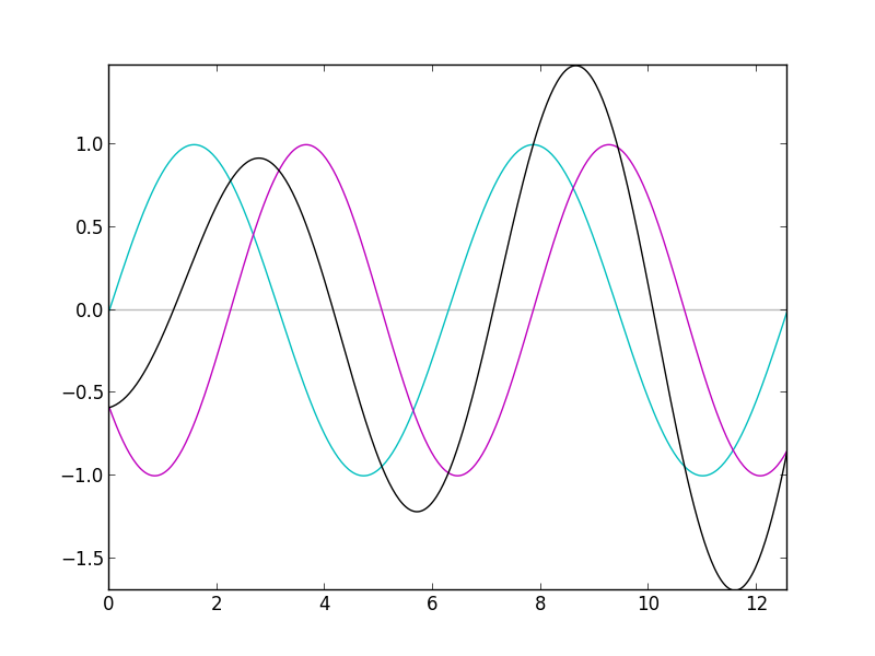
Phasing, rather simply, is the modification of a given signal by combining a copy of the signal with the original signal, wherein the copy is out of phase with the original. In the code shown, we haven't introduced an explicit phase shift, but because the second oscillator is playing at a slightly higher frequency than the first, it will go through cycles of being in phase, and out of phase with the original signal. The above image demonstrates the result (in black) for two simple sine waves at different frequencies. Notice that its amplitude changes between successive cycles.
With saw waves, this has a particularly interesting effect. To bring Fourier Series into the discussion, a saw wave can be represented as a sum of sine waves: one sine wave (referred to as a harmonic, or a partial) for each integer multiple of the fundamental frequency. The highest partial is at a very high frequency, and in the detuned copy, it plays at an even higher frequency. At that high frequency, this high harmonic goes through its periodic cycles of being in phase and out of phase quicker than the others. At a certain point, the detuned copy is 180° out of phase with the original, canceling out the original signal entirely. The second highest harmonic reaches that state just after the highest harmonic does. Then the third highest, the fourth highest, and so on. Thus the harmonics go in cycles of canceling themselves out all the way down the frequency spectrum, creating an interesting sweeping movement through the sound.
Now, recall earlier that I mentioned a third oscillator in my example: the sine wave oscillator. It's there to support the fundamental frequency because two saw waves playing out of phase with one another will eventually phase out the fundamental frequency, losing that powerful low end characteristic of these basses. By including a pure sine wave at the fundamental frequency, we ensure that the phasing we've introduced into the two sawtooth oscillators doesn't entirely cancel out our low end signal.
WaveShaping
Even though we’re just getting started, we already have a really versatile sound. But what good neuro bass would be complete without some distortion to really give those highs an edge and those lows some extra power?
In true signal processing, any perturbation of a given input signal is technically a type of distortion. Obviously, then, there are many different kinds of distortion. However, our discussion will largely pertain to harmonic distortion, characterized by the introduction of integer multiples of the input signal’s frequencies, as such distortion is generally musically pleasing.
The Web Audio API provides a simple but very effective utility for exploring various kinds of harmonic distortion: the WaveShaper node. In essence, the WaveShaperNode takes a function, f(x), known as a transfer function, and applies that function on its input signal to produce the output signal. This feature has almost limitless potential, but we'll be focusing on a couple of the more popular applications: clipping and saturation.
Update (12-15-2015): It's not entirely accurate to call the function f(x) here a transfer function, though for non-linear definitions of f the standard nomenclature is a little ambiguous. We could definitively say that the WaveShaperNode takes a function, f, such that, given input x, the output, y, is defined by y[n] = f(x[n]).
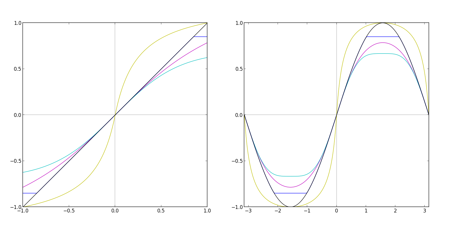
Clipping is a very common phenomenon in digital audio. Digital audio formats have strict bounds on the range the signal can occupy. For example, 16-bit and 24-bit WAV file formats carry signals on the range [-1, 1], thus if you were to write a sine wave signal with an amplitude greater than one to WAV format, the tip of the sine wave would be cut off in the resulting file. This is called "hard" clipping, and you can see an example of hard clipping (blue) applied to the original signal (black) in the diagram above. Considering that speaker cones can only move on small, fixed ranges, this detail of digital audio formats makes plenty of sense.
The sharp corners introduced by hard clipping create very harsh, aggressive forms of distortion, and usually introduces non-integer partials to the waveform to represent the sharp corners. In plenty of cases, this characteristic is desirable (guitar overdrive in the metal genre, and many dubstep bass sounds, for example). Some common forms of hard clipping distortion actually involve driving (amplifying) the input signal drastically before applying the hard clipping curve, to accentuate the sharp angle in the resulting waveform.
curve[i] = 0.5 * (Math.abs(x + 0.85) - Math.abs(x - 0.85));
This line, taken from my Waveshaper.js module, demonstrates a hard clipping WaveShaper curve, shown above in the left hand side of the chart by the blue line, and its effect is shown on the right hand side, again in blue. The magic number, 0.85, in this formula is the artificial limit at which we hard clip the input signal.
While the result of hard clipping is sometimes desirable, the process forfeits a lot of the information in your original signal, because any values greater than the clipping limit are thrown away (in this way, a hard clipper can act very much like a limiter). For this reason, and to reduce the harshness of hard clipping, "soft" clipping is often used as an alternative. Soft clipping, shown in the above graph in cyan and magenta, clips away the tips of the input signal, but does so with smoother corners. Though smoother, these corners still require high frequency partials, sometimes non-integer partials depending how sharp the clipping curve. A similar approach to yielding such a sound involves a simple low pass filter after a hard clipping curve to round out some of the sharper corners by removing the higher partials that make up the sharp curve.
curve[i] = Math.tanh(x);
curve[i] = Math.atan(x);
curve[i] = x - Math.pow(x, 3) / 4;
The formulas shown here, again from my WaveShaper.js module, each demonstrate soft clipping formulas. The first two are actually fairly classic saturation curves, whereas the third is a cubic approximation to Math.tanh(x). The approximation is drawn above in cyan, and Math.tanh(x) is drawn in magenta. Such approximation curves are used quite frequently due to the complexity of computing Math.tanh(x) in real time, although the Web Audio API's WaveShaper node skirts this problem by using a pre-calculated lookup table.
You'll notice that I referred to these curves both as soft clipping curves, and as saturation curves. The difference is often overlooked in modern "bedroom" producing. A true soft clipping curve is piecewise linear. It's very similar, in fact, to a hard clipping curve, except that in hard clipping, the "knee" is zero, meaning that as you exceed the clipping limit, the output signal is strictly capped to the clipping limit. In true soft clipping, the knee is non-zero; imagine, where the hard clipping curve goes flat, the soft clipping curve continues linearly with a non-zero slope of value less than one. The true difference, then, between soft clipping and saturation, is that saturation curves are non-linear. Thus, all of the "soft clipping" formulae I showed above are actually saturation curves. The audible difference is usually extremely slight, hence the common overlooking of such detail.
As a quick aside, I find it interesting to share a bit of the history of saturation curves. I mentioned above that hard clipping, at least historically, is due to the hard limit of the signal range supported by digital audio engines or file formats. Saturation, then, is historically a result of the signal range limits enforced by analogue tape. As values outside the supported range are written to analogue tape, the manner in which the tape breaks down is much less predictable than in the case of digital audio formats. Hence, the result is usually a non-linear function of the input signal, which we emulate with curves like the ones described above.
Now, there's one more curve in particular that we haven't discussed yet, which is actually the one I chose for this step of the sound design process. You'll find it shown on the graph in yellow, and used in the same WaveShaper.js module as follows.
curve[i] = (1 + k) * x / (1 + k * Math.abs(x))
I am unaware of the proper name for such a curve, but for the sake of this project, I'm referring to it simply as an S-Curve. In the above formula, k is a number value representing how aggressive the S-Curve shape is, or, how far it deviates from f(x) = x. Notice how the result of this curve applied to the input sine wave signal is not too different from the result of the soft clipping curves, save from the additional amplification. Indeed the effect it has on the sound is very similar as well: a slight edge (not too aggressive) in the higher end of the frequency spectrum, and some extra power on the lower end, just as we were aiming for.
This is now a good opportunity to step back and look at the higher level view of our sound design process. We have a simple, three oscillator synthesizer with interesting phasing characteristics resulting from detuned harmonic interaction and nice movement throughout the low end of the frequency spectrum, going through a single WaveShaper with an S-like curve shape, bringing character to the high end of the frequency spectrum and some power to the low end. If you're following along in the code, this is all represented in the function stepOne in the index.js module:
function stepOne(callback) {
  var bass = new Bass(ctx);
  var recorder = new RecorderWrapper(ctx);
  var ws = new WaveShaper(ctx, {amount: 0.6});
  var notes = [
    'g#1', 'g#1', '__', 'g#3',
    'g#1', 'g#1', '__', 'b2',
    'g#1', 'g#1', 'g#1', 'g#1',
    '__', 'g#2', '__', 'c#2'
  ];

  bass.connect(ws);
  ws.connect(recorder);
  ws.connect(ctx.destination);

  recorder.start();
  bass.play(BPM, 1, notes, function(e) {
    recorder.stop(callback);
  });
}
A quick look at this piece of the code reveals our next step: recording the output of the WaveShaper node as the bass plays through it. Tune back in shortly for part two, where we'll explore resampling, as it applies to using this recorded buffer, filter modulation, and take another high level look at how all of these pieces fit together to produce the finished sound.
Additional Reading: